Visualizing pathfinding Algorithms! BFS, DFS and A*

Visualizing Pathfinding Algorithms using Unity #

You can find the original twitter post this is based on here You can find the github project for this here

I always wanted to compare pathfinding algorithms, and was too busy to find a time. One night I started working on it, and in no time I had a tech demo ready.

Initial design #

My goal was to design a grid, in which I could position a character on any tile, position another character on a different tile, and then see the pathfinding algorithm in action. from the very first to the very last step. But first - some background

background #

First, let’s remember how DFS, BFS and A* work

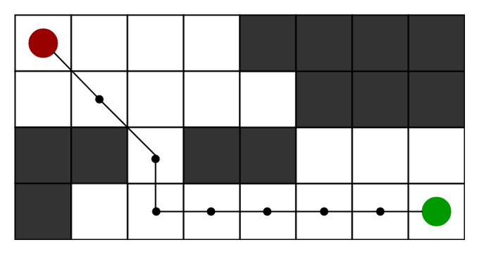
DFS #

DFS algorithm starts at the root (top) node of a tree and goes as far as it can down a given branch (path), then backtracks until it finds an unexplored path, and then explores it. The algorithm does this until the entire graph has been explored.

Simply put, every tile in our grid is a node in the graph. Every node has 8 different other nodes it can explore. The character is at the starting node, so DFS acts accordingly

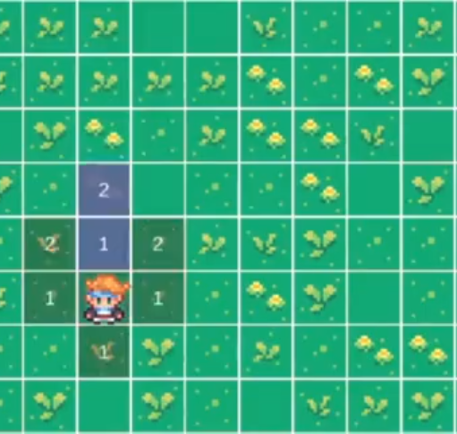
it picks a neighbor node and goes deeper:

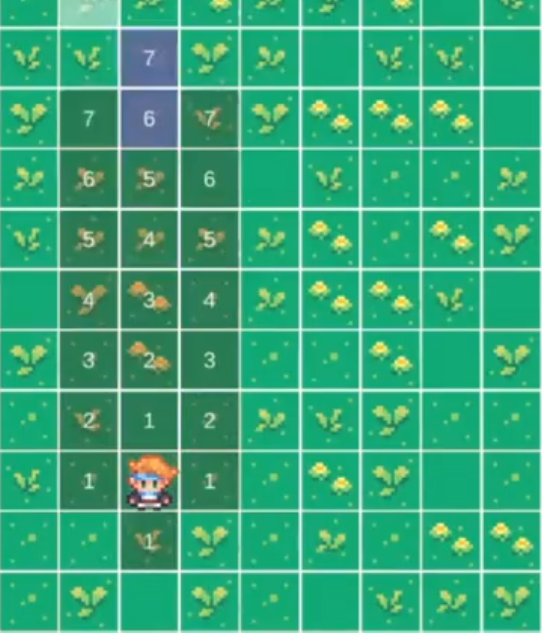
it keeps going deeper (Hence - depth-first-search) until the target is reached - but the path is very long

BFS (Dijkstra with weights=1) #

BFS algorithm starts at the root (top) node and explores the graph layer by layer, examining all the nodes at the same level before descending further. It uses a queue data structure to maintain the order of exploration, ensuring that nodes are visited in a breadth first manner. here’s a useful link on Dijkstra if you want to remember why it’s the same as BFS when weights=1

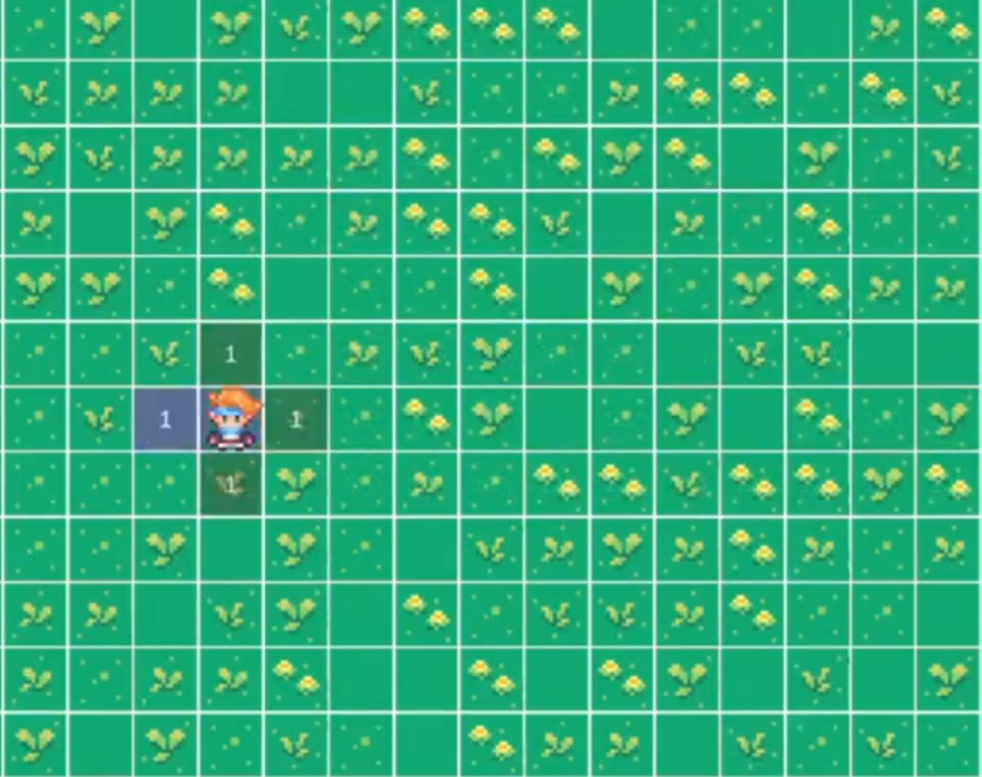
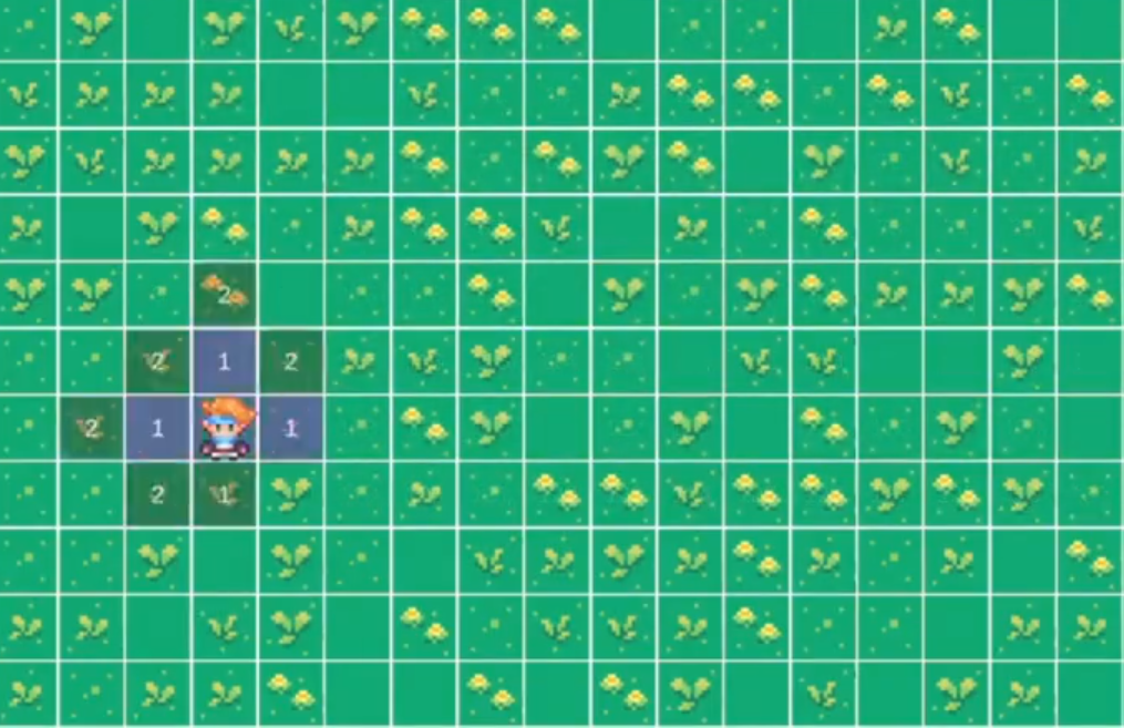
Simple put, we always visit every neighbor of the node before continuing to the next node.

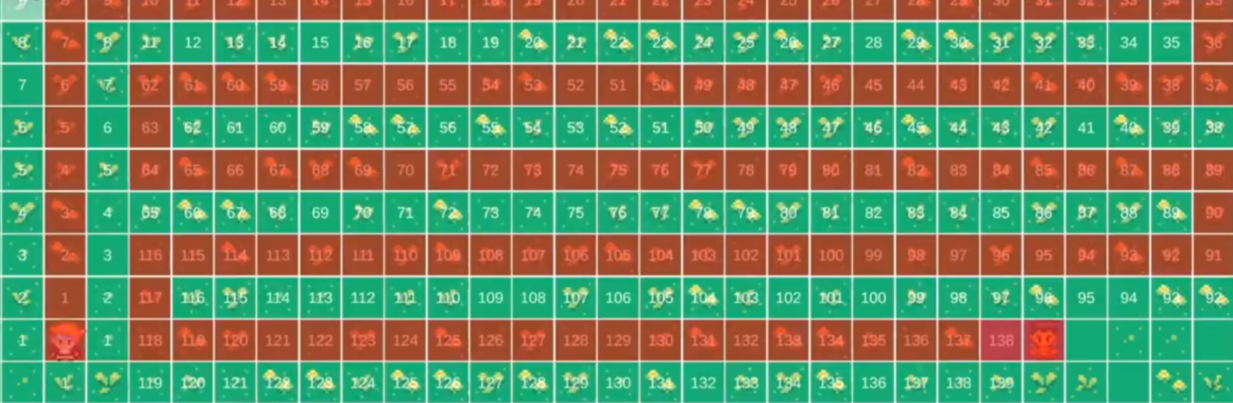
This is how BFS does this. The blue nodes are currently inside the queue, waiting to be explored.

and now we explore the outer nodes:

And so on:

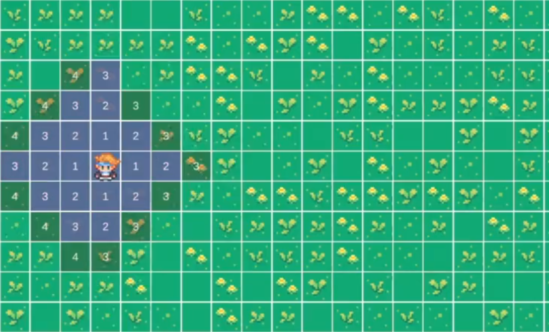
and so on:

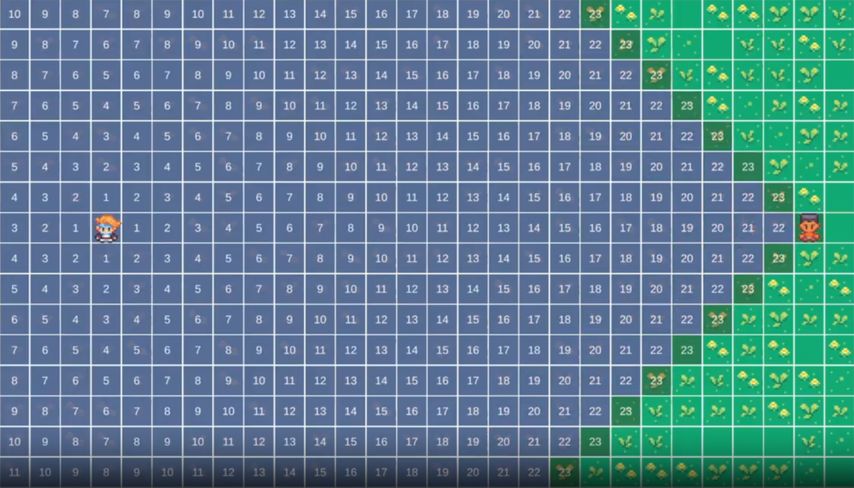
Until:

A* #

Similar to BFS, but at any step on the grid, A* calculates not only the length so far by simply scanning the grid (similar to BFS), A* adds another step where it calculates the distance (Manhattan)

Straightforward Comparison - No Limitations #

As a first comparison, I placed them on an open grid, without any walls. It is noteworthy that although DFS promises to find a path but does not guarantee it will be the shortest, BFS (Dijkstra) guarantees to find the shortest path but does not guarantee the computation time, and A* “guarantees” (heuristic) to find the shortest path and in the quickest amount of time. How quick? incredibly quick. Here’s a video comparison all three. In the left corner you can see which algorithm is currently running.

Why does A* performs so much better then the other two? #

A* performs much better because of the main difference it has from the other two - it not only calculates the nodes it already knows, it calculates the distance from the final node.
This simple heuristic improves the algorithm dramatically in the clean case we just saw, but it can also lead to a worse results in different scenarios.

Adding A Maze #

Then I started complicating things even more. I placed them in a random maze I created, and wanted to see who will win. A* won, but mostly because it can “give up” on certain paths, where BFS never gives up on any path. Here’s another video comparison of all three. In the left corner you can see which algorithm is currently running.

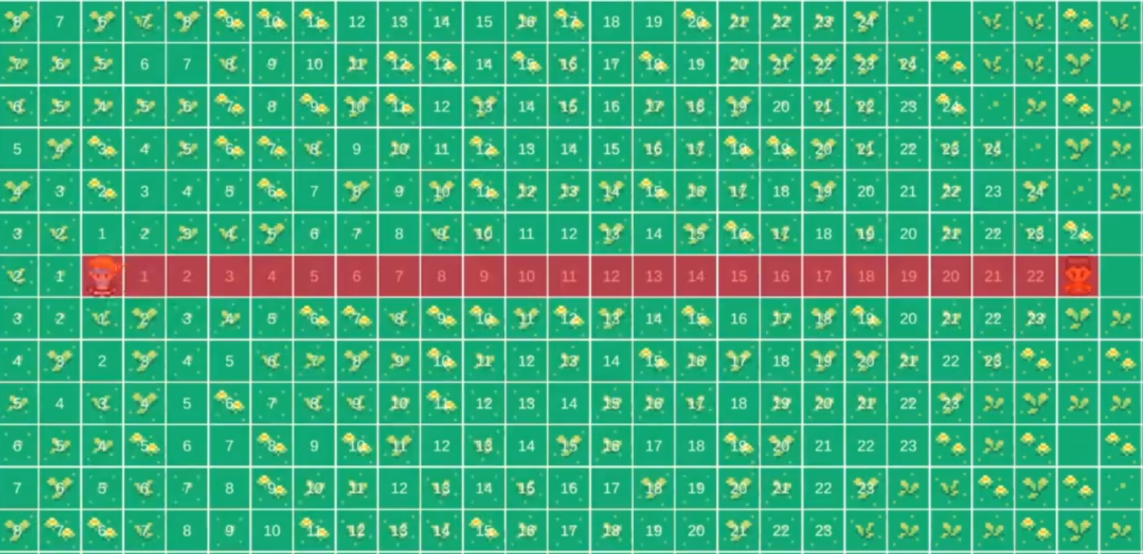
Where A* Fails #

Although it may appear that I give A* too much credit, there are instances in which it falls short
The best example I found was when I placed the end node behind a wall.
A* performs miserably since the distance calculation throws it off, and it doesn’t “give up” those very close steps it believes that lead him to the his final destination.

Conclusion #

Although it seems like A* is the best choice, there are many cases (not just the one I shared) where BFS and even DFS can perform better. When adding weights, the whole story changes, but more on that in a future post.